? Boo

In a term project picked up from my York colleague Paul Delaney, undergraduate non-science majors in my intro astro class photograph a constellation.  While doing so last fall, one student may have discovered a previously unknown flare star in Bootes, flaring to 5th magnitude next to omicron Boo and pi Boo.  We have dubbed this object "? Boo".

Details are available at http://www.aavso.org/possible-flare-star-bootis ...including a link to astrometry.net where I was able to get an astrometric calibration of the field:
http://nova.astrometry.net/user_images/tag?thumbnail_size=&sort=&calibrated=on&failed=on&query=Bootes+Flare

Being busy with other projects, I'm restraining myself from trawling through online archival databases to look for evidence of variability in either of the two candidate stars that might have hosted this flare.

Another thing to restrain myself from (for a while) is to take the 1/8th second exposure handheld image, in which the stars have the shape of a seeing disk trailed in a complicated pattern due to jitter, and see if I can get better astrometry from it than from the 2 second exposure, in which the stars have the shape of a seeing disk trailed over and over itself until it's just a blurry blob.  By isolating the brightest part of each star in the 1/8th second image, it may be possible to measure the astrometric position of ? Boo to the limit allowed by seeing or pixel size rather than by handheld blurring.  Speckle interferometry on the cheap!  And if you're reading this and are intrigued by this idea, go ahead and try it!

Marching On

Too long since my last post!  Since which I have:

* noticed a new flare star in Bootes (of which more anon)

* worked with undergrad students Erik Weiss and Amanda DeSouza on using current observations of accretion disk sizes as a function of wavelength to constrain their temperature profiles, and thought with grad student Laura Chajet about what might produce such profiles

* plugged away on the referee report for my paper on redshifted-trough BAL quasars (so close...)

* prepared observation templates for the Gemini 8-meter telescopes, did quick-look reductions on some spectra, and helped grad student Jesse Rogerson get started on real reductions

* taught astronomy

* helped write proposals for the Hubble Space Telescope and the Chandra X-ray observatory

* started thinking about proposals for Gemini and the 3.6-meter Canada-France-Hawaii Telescope

Back to work...

CFHT quick-look

[Technical post about ongoing project.]


To examine colours of one quasar in CFHT imaging:

Locate g, r, i images of quasar. [in this example, they are 1571 + 386p, 397p, 408p]


Create coordinates file of comparison stars on same chip which are not saturated in any filter and thus can be used to calculate the aperture correction in all filters:

photcal> head j224733.coo.1
1066 1271
1204 3015
208 2956
686 1348
521 1321


Create coordinates file of quasar:

photcal> head j224733.coo.2
752 1385

In IRAF, load noao.digiphot, type "datapars", and make sure these parameters are set:

(ccdread=              RDNOISE) CCD readout noise image header keyword
(gain   =                     ) CCD gain image header keyword
(readnoi=                   0.) CCD readout noise in electrons
(epadu  =                   1.) Gain in electrons per count
(exposur=              EXPTIME) Exposure time image header keyword
(airmass=              AIRMASS) Airmass image header keyword

(filter =               FILTER) Filter image header keyword

In photpars, I set:
apertur= 5,7.5,10,12.5,15,17.5,20,22.5,25,27.5,30,35,40,45,50
which I recommend doing, to help identify any outlier stars in the aperture correction phase.

Photometer comparison stars & quasars separately:
(I couldn't get e.g. "phot 1571386p.fits[ccd03]" to work, so I first copied the extensions to individual images, but I see now that I should have just done "phot 1571386p.fits[3]".) 

imcopy 1571386p.fits[ccd03] 1571386p03.fits
phot 1571386p03.fits coo=j224733.coo.1 interac-
phot 1571386p03.fits coo=j224733.coo.2 interac-

imcopy 1571397p.fits[ccd03] 1571397p03.fits
phot 1571397p03.fits coo=j224733.coo.1 interac-
phot 1571397p03.fits coo=j224733.coo.2 interac-

imcopy 1571408p.fits[ccd03] 1571408p03.fits
phot 1571408p03.fits coo=j224733.coo.1 interac-
phot 1571408p03.fits coo=j224733.coo.2 interac-

Use output to calculate aperture correction between aperture 1 (5 pixels) and aperture 9 (25 pixels) using the "mkapfile" task in the "photcal" package in noao.digiphot:

mkapf 1571386p03.fits.mag.1  9 1571386p03.apcor.1 small=1 large=9

mkapf 1571397p03.fits.mag.1  9 1571397p03.apcor.1 small=1 large=9 nparams=2

mkapf 1571408p03.fits.mag.1  9 1571408p03.apcor.1 small=1 large=9

[r-band apcor wouldn't converge unless number of free parameters was reduced]



Extract quasar magnitude and apply aperture correction in each filter (all IRAF commands):
#g:
txdump 1571386p03.fits.mag.2 mag yes | scan (x)
txdump 1571386p03.fits.mag.2 merr yes | scan (y)
fields 1571386p03.apcor.1 3 | sort num+ rev+ | scan (z)
y=sqrt(y**2.+z**2.)
fields 1571386p03.apcor.1 2 | sort num+ rev+ | scan (z)
x=x+z
printf("%7.3f %6.3f %8.3f\n",x,y,z, >> "1571386p03.mea")
#r:
txdump 1571397p03.fits.mag.2 mag yes | scan (x)
txdump 1571397p03.fits.mag.2 merr yes | scan (y)
fields 1571397p03.apcor.1 3 | sort num+ rev+ | scan (z)
y=sqrt(y**2.+z**2.)
fields 1571397p03.apcor.1 2 | sort num+ rev+ | scan (z)
x=x+z
printf("%7.3f %6.3f %8.3f\n",x,y,z, >> "1571397p03.mea")
#i:
txdump 1571408p03.fits.mag.2 mag yes | scan (x)
txdump 1571408p03.fits.mag.2 merr yes | scan (y)
fields 1571408p03.apcor.1 3 | sort num+ rev+ | scan (z)
y=sqrt(y**2.+z**2.)
fields 1571408p03.apcor.1 2 | sort num+ rev+ | scan (z)
x=x+z
printf("%7.3f %6.3f %8.3f\n",x,y,z, >> "1571408p03.mea")

head 1571*p03.mea
===> 1571386p03.mea <=== -6.1195  0.023   -0.307 g
===> 1571397p03.mea <=== -6.374  0.014   -0.178 r
===> 1571408p03.mea <=== -6.437  0.014   -0.214 i

Table of values useful for calculating calibrated magnitudes:

filter              g       r       i
exptime 52.071  85.049  144.052
X_?        1.295   1.225   1.153
?_c       26.485  26.020  25.840
?_c_err 0.0098  0.0076  0.0070
?_X        0.148   0.0     0.0830
?_K       -0.15   -0.10   -0.040
g,r,i     -6.1195 -6.374  -6.437


Calculate calibrated magnitudes; R then G then I:

#R = r + r_c + r_K*(X_r-1)
= -6.374 + 26.020 -0.10*0.225   # 19.624
#Rerr
= sqrt(0.014**2.+0.0076**2.)    #  0.016
#G
=(-6.1195 + 26.485 + -0.15*0.295 - 0.148*19.624)/(1-0.148) # 20.442
#Gerr
= sqrt(0.023**2.+0.0098**2.)    #                                             0.025
#I
=(-6.437+25.840+ -0.04*0.153 +0.083*19.624)/(1+0.083) #  19.414
#Ierr
= sqrt(0.014**2.+0.0070**2.)    #                                          0.016

G         R         I
20.442 19.624 19.414
+-0.025  0.016  0.016

=20.442-19.624; = sqrt(0.025**2.+0.016**2.) #G-R & err
=19.624-19.414; =sqrt(0.016**2.+0.016**2.) #R-I & err

G-R = 0.82 +- 0.03
R-I = 0.21 +- 0.02

These values match those observed in Stripe 82 for this quasar.  No evidence that the blue shape of the BOSS spectra in between S82 and CFHT epochs is real.

(A check of one comparison star confirms that the CFHT magnitude scale is close enough to the SDSS magnitude scale that the above conclusion will not be invalidated by systematic errors.)

Podcast

Check out an interview with me on the Star Spot Podcast!  (I apologize in advance for my audio fading in and out.  Maybe I should just speak loudly and excitedly all the time!  Whatever the solution, clearly I need more practice keeping my voice evenly modulated in interviews.)

Both Sides Now

PSU grad student Nur Filiz Ak led a project that watched clouds (of a sort) clear out from in between us and some distant black holes... cool to be part of that. http://www.sdss3.org/press/thewind.php

And we just submitted a proposal to look at clouds that have appeared in quasar spectra.  We think the clouds are moving into and out of our line of sight.  If approved, our recent proposal means we'll have looked at the leading and trailing sides of clouds, hence the title of this post...

Length of the Seasons, 2011-2012

Fun fact: because Earth's perihelion currently occurs in early January, it is moving faster in its orbit during northern hemisphere fall and winter.  So the northern hemisphere currently gets a week more spring+summer than fall+winter.

---

Behold the math:

In 2011-2012, length of the northern hemisphere seasons in minutes:

winter:
Dec 22 05 30 to Dec 31 24 00 plus
Jan 01 00 00 to Mar 20 05 14: = (9*24+18.5)*60 + ((31+29+19)*24+(5+14/60.))*60
128144.

spring:
Mar 20 05 14 to Jun 20 23 09: = ((11+30+31+19)*24+(18+46/60.+23+9/60.))*60
133555.

summer:
Jun 20 23 09 to Sep 22 14 49: = ((10+31+31+21)*24+(0+51/60.+14+49/60.))*60
134860.

fall:
Sep 22 14 49 to Dec 21 11 12: = ((8+31+30+20)*24+(9+11/60.+11+12/60.))*60
129383.

ecl> =128144+129383-134860-133555
-10888
ecl> =10888/(24*60.)
7.5611111111111

sanity check:
=(128144+129383+134860+133555)/(24*60.)
365.2375

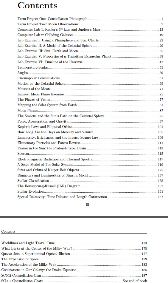
Astronomy Activities Manual

Last month saw the publication of my "Astronomy Activities Manual" from Kendall Hunt. If you're looking for in-class activities and a few lab exercises and assignments for students in your undergrad intro astro class, Kendall Hunt has published a wide of activities by numerous authors over the years. You can pick and choose the ones you like and put them together into a custom workbook (and the authors get royalties). I've taken existing activities that I think will work well in my class and added a dozen or so of my own, mostly for the extragalactic half of the course. If you're interested, check out the table of contents below and contact Richard Ludlow at Kendall Hunt (rludlow At kendallhunt.com) to get a sample copy.  (PS - it's not a typo; there is no Lab IV in the book.)